知乎原帖复现
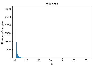
1
2
3
4
5
x_min = 1 alpha = 3.5 rnd_list = np.random.uniform(0 , 1 , 10 **5 ) x_list = x_min * np.power(1 - rnd_list, -1 / (alpha - 1 ))
原始数据直方图
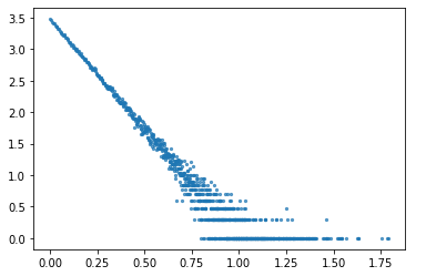
log-log图
log-log图
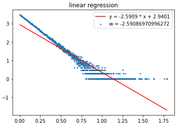
经过线性回归的log-log图
$$ \alpha = 2.59 \tag{1} $$
经过指数/对数分箱之后,进行了参数估计 这里在分箱之前没有处理,所以最后得到的alpha = -w + 1的
从原贴看出,作者在最后进行参数估计的时候,将分箱的数量大大减少。
$$ \alpha = 3.50 \tag{2} $$
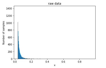
转化到0-1
思路 由原帖,推知的幂律分布公式:$ x = x_{min}(1-r)^{-1\over -(\alpha-1)} $,因为要得到$ x \in (0, 1)$, 所以就是要求函数r的定义域,但是发现比较难求,转换为求原始函数$ r = 1-({x\over x_{min}})^{-(\alpha-1)}$的在$ x \in (0, 1)$的值域。
发现在$ r < 0$时,$ x \in (0, 1)$。
这里有一个问题就是 :对这个负值的取值问题 负值的取值,与随机出来的幂律分布的下限存在一定关系。负值取得越小越接近零,但是其上限可能也会随之减小。
大样本的尝试 1 2 3 4 5 6 7 参数 r (-5000 , 0 )---------------------幂律分布的最大最小值0.03314199326291829 0.9516629536071909 bin = 5000 rnd_list = np.random.uniform(-5000 , 0 , 10 **5 ) 0.03314199326291829 0.9516629536071909 intervals = np.logspace(-2 , 0 , 100 , base = 10 )
原始数据
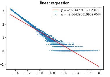
均匀分箱:log-log图以及线性回归
大样本均匀分箱:$$ \alpha = 2.66 \tag{3} $$
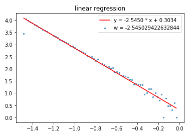
指数/对数分箱:参数估计
大样本指数/对数分箱:$$ \alpha = 3.54 \tag{4} $$
小样本尝试 1 2 3 4 5 参数 bin = 500 rnd_list = np.random.uniform(-5000 , 0 , 2000 ) 0.033144970720553266 0.6949274551386315 intervals = np.logspace(-1.5 , 0 , 15 , base = 10 )
原始数据
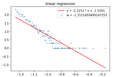
均匀分箱:log-log图以及线性回归
小样本均匀分箱:$$ \alpha = 2.31 \tag{5} $$
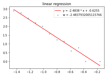
指数/对数分箱:参数估计
小样本指数/对数分箱:$$ \alpha = 3.48 \tag{6} $$
源码 1 2 3 4 5 6 7 8 9 10 11 12 13 14 15 16 17 18 19 20 21 22 23 24 25 26 27 28 29 30 31 32 33 34 35 36 37 38 39 40 41 42 43 44 45 46 47 48 49 50 51 52 53 54 55 56 57 58 59 60 61 62 63 64 65 66 67 68 69 70 71 72 73 74 75 76 77 78 79 80 81 82 83 84 85 86 87 88 89 90 91 92 93 94 95 96 97 98 99 100 101 102 103 104 105 106 107 108 import numpy as npimport mathimport randomfrom sklearn import linear_modelimport matplotlib.pyplot as pltx_min = 1 alpha = 3.5 rnd_list = np.random.uniform(0 , 1 , 10 **5 ) print (rnd_list)x_list = x_min * np.power(1 - rnd_list, -1 / (alpha - 1 )) print (x_list)hist_h, hist_x = np.histogram(x_list, bins=5000 ) print (len (hist_h))print ()plt.title('raw data' ) plt.xlabel('x' ) plt.ylabel('Number of samples' ) plt.hist(x_list, bins=5000 ) plt.show() y = hist_h x = [] pre = 0 for current in range (1 , len (hist_x)): xt = (hist_x[pre] + hist_x[current]) / 2 x.append(xt) pre = current print (len (x))start = 0.5 log_x = np.log10(x) log_y = np.log10(y) plt.scatter(log_x[0 :5000 ], log_y, s=5 , alpha=0.7 ) plt.show() reg_x = [] reg_y = [] for i, j in zip (log_x, log_y): if (not np.isinf(i)) and (not np.isinf(j)): reg_x.append([float (i)]) reg_y.append(float (j)) regr = linear_model.LinearRegression() regr.fit(reg_x, reg_y) w = regr.coef_ b = regr.intercept_ item = 'y = %.4f * x + %.4f' %(w[0 ], b) print (item)plt.title('linear regression' ) plt.scatter(log_x[0 :5000 ], log_y, s=5 , alpha=0.7 ) plt.plot(reg_x, regr.predict(reg_x), color='red' ) plt.legend(labels=[item, 'w = ' + str (w[0 ])], loc='upper right' ) plt.show() intervals = np.logspace(0 ,np.log10(100000 +10 ),100 ,base = 10 ) print (len (intervals))hist_h1, hist_x1 = np.histogram(x_list, bins=intervals) y1 = hist_h1 x1 = [] pre = 0 for current in range (1 , len (intervals)): xt = (intervals[pre] + intervals[current]) / 2 x1.append(xt) pre = current print (len (x))start = 0.5 log_x1 = np.log10(x1) log_y1 = np.log10(y1) plt.scatter(log_x1, log_y1, s=5 , alpha=0.7 ) plt.show() reg_x1 = [] reg_y1 = [] for i, j in zip (log_x1, log_y1): if (not np.isinf(i)) and (not np.isinf(j)): reg_x1.append([float (i)]) reg_y1.append(float (j)) regr1 = linear_model.LinearRegression() regr1.fit(reg_x1, reg_y1) w = regr1.coef_ b = regr1.intercept_ item = 'y = %.4f * x + %.4f' %(w[0 ], b) print (item)plt.title('linear regression' ) plt.scatter(log_x1[0 :5000 ], log_y1, s=5 , alpha=0.7 ) plt.plot(reg_x1, regr1.predict(reg_x1), color='red' ) plt.legend(labels=[item, 'w = ' + str (w[0 ])], loc='upper right' ) plt.show()